Automatic Control Example Series: A State Feedback Controller Using Ball Balancing Table
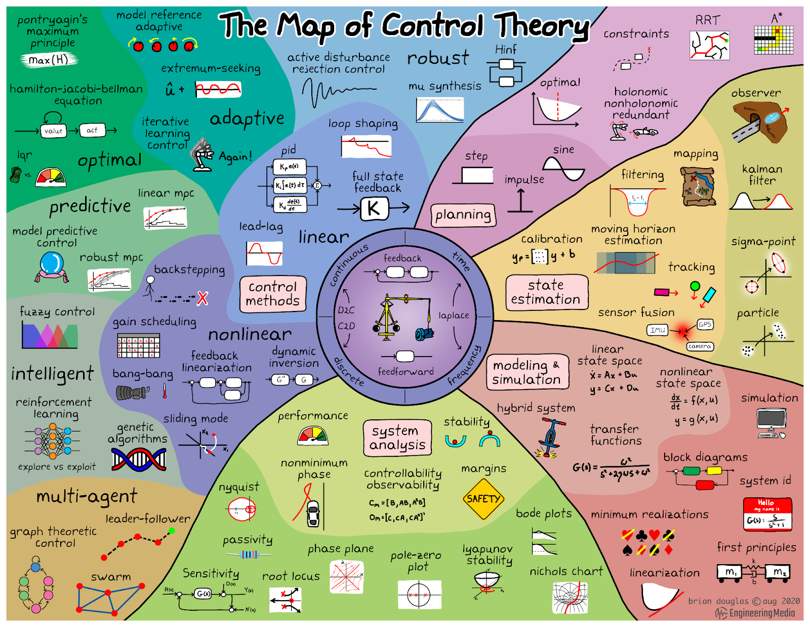
The field of Control Theory encompasses numerous methodologies and applications, eloquently outlined and categorized by Brian Douglas on his blog page at Engineering Media.
Within this series of blog documents, we aim to implement several of these control theory topics utilizing Acrome's accessible control and robotics experiment systems. Examples include Reinforcement Learning, Kalman Filters, LQR/LGQ controllers, and Stability and Bode Plots.
This particular blog focuses on a project employing The Ball Balancing Table to illustrate a State Feedback controller. This post will delve into the foundational aspects of both the hardware and the underlying algorithm.
Details of Hardware and Software:
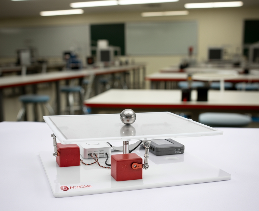
Introduction to the Ball Balancing Table (BBT)
The Ball Balancing Table is a classic experiment in control systems that bridges academic topics (esp. the control theory) with the industrial processes and projects. It consists of a flat surface (the table) where a ball is placed, and the objective is to control the tilt of the table to guide the ball to specific locations on this table.
Users/students can learn control concepts -like State Feedback- but also can do simpler or more complex experiments with different types of controllers, such as PID, and reinforcement learning. The open-source software methodology allows users to modify and test advanced control algorithms, change the controllers or other system parts which makes it a versatile tool for both academic and real-world applications.
State Feedback Controller Basics
What is a State Feedback Controller?
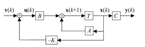
A state feedback controller is a control approach where the control action is based on the entire set of state variables of the system, not just the output. By feeding back the system’s states, it allows direct adjustment of the system dynamics, such as stability and response speed. This method gives the designer more flexibility, especially for modern control techniques, and is often combined with observers when not all states are measurable.
What is Pole Placement?
Using output or state feedback, the poles or eigenvalues of the system can be assigned subject to system-dependent limitations. This is known as pole placement, pole assignment, or pole allocation. System poles are determined according to the system's overshoot and settling time requirements.
The dynamics of the closed-loop system depend on the eigenstructure (eigenvalues and eigenvectors) of the matrix Acl. Thus, the desired system dynamics can be chosen with appropriate choice of the gain matrix K.
If the pair (A,B) is controllable, then there exists a feedback gain matrix K. It is evaluated the desired characteristic polynomial from specified eigenvalues.
Implementing the State Feedback Controller Example
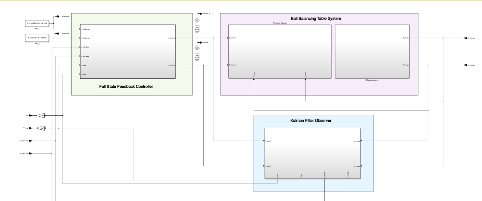
The State Feedback Controller Example is implemented using Matlab® and Simulink® software of The Mathworks™ and the Acrome’s Ball Balancing Table as a student intern project led by the author of this article. Full application codes are available on request.
The Acrome Ball Balancing Table system consists of two servo motors and a touchscreen sensor. The angle applied by the servo motors is input to the system. The output of the system is the speed and position values in the x and y axes. The system contains multiple state variables (speed and position). A full-state feedback controller is very useful in such systems.
Controllers that only look for errors, such as PIDs, are not fast or stable enough in such systems. Position and velocity are evaluated simultaneously with full-state feedback. The desired system dynamics (overshoot, settling time, etc.) are achieved through pole placement. Unmeasurable situations can be predicted using an observer.
The controller measures, observes, or performs both of the state variables in the system and multiplies them by the calculated K-matrix gain, thus entering them into a feedback loop. How to calculate the K-matrix gain was discussed in the previous section. The purpose of this is to achieve stability and rapid response by controlling all dynamics of the system simultaneously.
What we want to balance: a ball resting on a platform
Inputs: Angles of the servo motors tilting the platform
Outputs: x and y positions of the ball
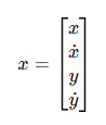
State variables: x, ẋ (position and velocity in the x-direction) y, ẏ (position and velocity in the y-direction)
So, our state vector is:
Using this information and the available input and output blocks of the BBT, we are now ready to implement our controller example in software.
State Feedback Controller Design and Simulation Example Matlab Code
% System matrices (X axis)
A_x = [0 1;0 0];
B_x = [0; 1.142];
C_x = [1 0];
D_x = 0;
% System matrices (Y axis)
A_y = [0 1;0 0];
B_y = [0; 1.42];
C_y = [1 0];
D_y = 0;
% Design specifications
overshoot = 5; % overshoot
zeta = -log(overshoot/100) / sqrt(pi^2 + (log(overshoot/100))^2); % damping ratio
T_s = 3; % settling time [s]
wn = 4/(T_s*zeta); % natural frequency
wd = wn*sqrt(1 - zeta^2); % damped natural frequency
sigma = 4/T_s; % real axis value for pole placement
desired_poles = [-sigma+1j*wd, -sigma-1j*wd];
desired_poles_x = desired_poles;
desired_poles_y = desired_poles;
% Reference gain calculation (precompensator)
A_cl_x = A_x - B_x*K_x;
G_ss_x = -C_x * (A_cl_x \ B_x); % use backslash instead of inv
N_x = 1 / G_ss_x;
fprintf('N_x = %.6f\n', N_x);
A_cl_y = A_y - B_y*K_y;
G_ss_y = -C_y * (A_cl_y \ B_y);
N_y = 1 / G_ss_y;
fprintf('N_y = %.6f\n', N_y);
% Closed-loop systems (with state feedback + reference gain)
Acl_x = A_x - B_x*K_x;
Bcl_x = B_x*N_x;
Ccl_x = C_x;
Dcl_x = 0;
sys_cl_x = ss(Acl_x, Bcl_x, Ccl_x, Dcl_x);
Acl_y = A_y - B_y*K_y;
Bcl_y = B_y*N_y;
Ccl_y = C_y;
Dcl_y = 0;
sys_cl_y = ss(Acl_y, Bcl_y, Ccl_y, Dcl_y);
% Simulation time
t = 0:0.01:6;
r = ones(size(t)); % step input
% Step responses
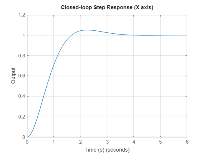
figure;
step(sys_cl_x, t);
title('Closed-loop Step Response (X axis)');
xlabel('Time (s)');
ylabel('Output'); grid on;
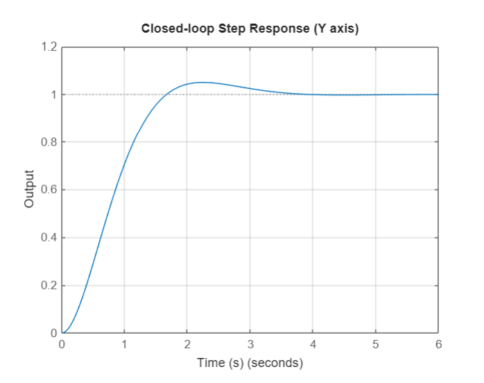
figure;
step(sys_cl_y, t);
title('Closed-loop Step Response (Y axis)');
xlabel('Time (s)'); ylabel('Output'); grid on;
% State trajectories (X axis)
[x_out_x, t_x, x_states_x] = lsim(sys_cl_x, r, t, [0;0]);
figure;
plot(t_x, x_states_x(:,1), 'r-', 'LineWidth', 1.5); hold on;
plot(t_x, x_states_x(:,2), 'b--', 'LineWidth', 1.5); l
egend('x_1 (position)','x_2 (velocity)');
title('State trajectories (X axis)');
xlabel('Time (s)');
ylabel('States'); grid on;
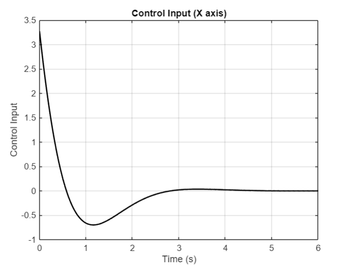
% Control input (X axis)
u_x = - (K_x * x_states_x')' + N_x * r';
figure;
plot(t, u_x, 'k', 'LineWidth', 1.5);
xlabel('Time (s)');
ylabel('Control Input');
title('Control Input (X axis)'); grid on;
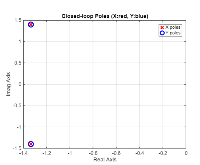
% Closed-loop pole locations
poles_x = eig(Acl_x);
poles_y = eig(Acl_y);
figure;
plot(real(poles_x), imag(poles_x), 'rx', 'MarkerSize', 10, 'LineWidth', 2); hold on; plot(real(poles_y), imag(poles_y), 'bo', 'MarkerSize', 10, 'LineWidth', 2);
xline(0,'--k');
xlabel('Real Axis'); ylabel('Imag Axis');
title('Closed-loop Poles (X:red, Y:blue)');
legend('X poles','Y poles'); grid on;
fprintf('N_y = %.6f\n', N_y);
figure;
step(sys_cl_x, t);
title('Closed-loop Step Response (X axis)');
xlabel('Time (s)'); ylabel('Output'); grid on;
figure;
step(sys_cl_y, t);
title('Closed-loop Step Response (Y axis)');
xlabel('Time (s)'); ylabel('Output'); grid on;
State Feedback Controller Example Result Graphs:

Conclusion
This blog post provides a comprehensive overview of implementing a State Feedback Controller using Acrome's Ball Balancing Table. It details the hardware and software aspects, explains the fundamental concepts of state feedback control and pole placement, and presents a practical implementation example using MATLAB and Simulink. The provided code snippets and resulting graphs demonstrate the design and simulation of the controller, showcasing its effectiveness in achieving desired system dynamics for the Ball Balancing Table. This example serves as a valuable resource for understanding and applying modern control techniques in real-world scenarios.
Contact ACROME to learn more about different control and robotics products and different engineering applications that can be done.
REFERENCES
[1] “The Map of Control Theory | Engineering Media” https://engineeringmedia.com/maps
[2] Brian L. Stevens; Frank L. Lewis; Eric N. Johnson. Aircraft control and simulation: Dynamics, controls design, and autonomous systems, 3rd edition. John Wiley & Sons Inc, 2016.
[3] “State Feedback - an Overview | ScienceDirect Topics.” www.sciencedirect.com/topics/engineering/state-feedback.
Author
