Sensor Drift Correction with Symbolic AI Using OpenMathAI

Summarize with:

A control experiment can fail before the controller is even tuned. If the attitude estimate delivered by an inertial measurement unit (IMU) moves when the physical platform is stationary, the controller reacts to an error that does not exist. On a twin-rotor 3-DoF platform, this problem becomes visible as soon as the motors run. Vibration couples into the accelerometer, motor currents disturb the magnetometer, and small gyroscope biases become angle errors after integration.

This article examines sensor drift correction at the sensor level. It focuses on the BNO055-based measurement chain used with the Acrome 3-DoF Copter, rather than repeating a general Kalman-filter tutorial. The practical question is narrower: how can logged real-hardware data reveal a repeatable, nonlinear correction, and when is a symbolic model a better engineering tool than another round of hand-tuned filtering?

The answer is not to discard sensor fusion. The BNO055 already combines a triaxial accelerometer, gyroscope, and magnetometer and can expose fused orientation, gravity, and linear-acceleration outputs1. A useful workflow instead separates three layers: physical calibration, baseline estimation, and a data-driven residual correction. Symbolic AI can operate on the residual layer, where it learns a compact equation for the error produced by vibration, motor state, temperature, or magnetic disturbance.

‍

Why the 3-DoF Copter’s IMU Drifts

The BNO055 is an intelligent 9-axis sensor, not a perfect attitude reference. Its NDOF mode combines accelerometer, gyroscope, and magnetometer measurements, while IMU mode uses accelerometer and gyroscope data without magnetic heading. A calibration status for each sensor does not mean that dynamic disturbances have disappeared 1 2.

For a control engineer, the measurement should be written as a model with errors:

‍

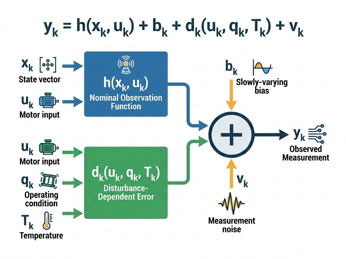
Diagram visualizing the measurement model equation y_k = h(x_k, u_k) + b_k + d_k(u_k, q_k, T_k) + v_k. Illustrates state x_k and motor input u_k feeding into nominal observation function h, summed with slowly-varying bias b_k, disturbance-dependent error d_k (taking inputs u_k, operating condition q_k, and temperature T_k), and measurement noise v_k to produce the observed measurement y_k.

Here, (xk) is the true attitude state, (uk) contains motor commands, (qk) represents vibration or operating condition, (Tk) is temperature, (bk) is a slowly varying bias, (dk) is a disturbance-dependent error, and (vk) is measurement noise. A conventional filter usually models (bk) and (vk) well. It may not model the structured term (dk), especially when the error changes with rotor speed and platform pose.

‍

Motor Vibration and the Accelerometer

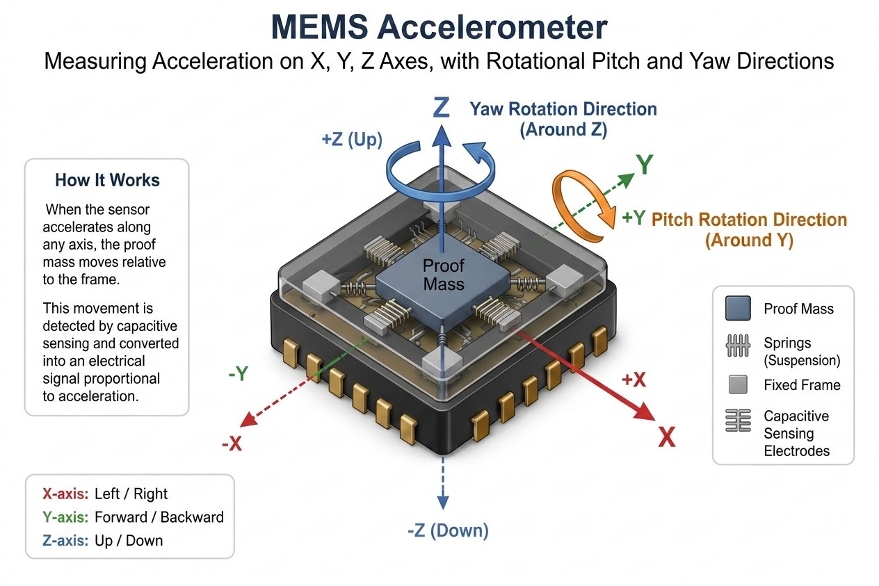
A MEMS accelerometer measures specific force. In a stationary test, its dominant signal is the gravity vector. During operation, the sensor also sees structural acceleration caused by the rotor arms, motor imbalance, bearing motion, and the platform’s mechanical modes.

A simplified measurement model is: a_m = S_aR_sb(a_b - g_b) + b_a + n_a

where S_a is the scale and cross-axis matrix, R_sb maps the body frame to the sensor frame, a_b is body acceleration, g_b is gravity, b_a is accelerometer bias, and n_a is noise. The vibration component is not necessarily white noise. It can contain harmonics related to motor speed and resonant peaks from the mechanical structure.

This distinction matters because the fusion algorithm may interpret high-frequency vibration as a short-lived change in the gravity direction. If the vibration is asymmetric across operating points, a fixed low-pass filter creates a trade-off. A lower cutoff reduces jitter but adds phase lag. A higher cutoff preserves response but allows more disturbance into the attitude estimate. The BNO055 provides selectable bandwidth settings for both accelerometer and gyroscope channels, so bandwidth is an experimental variable rather than a hidden constant 1 2.

Log acceleration, fused angle, motor command, and encoder angle together. A power spectral density comparison across motor speeds can reveal peaks that move with the operating point, indicating structured vibration coupling.

‍

Magnetic Interference from the Rotors

The magnetometer is especially vulnerable to the hardware around it. A current-carrying conductor produces a magnetic field, and a motor assembly adds permanent-magnet and ferromagnetic effects. The resulting field is the sum of the Earth field, hard-iron offset, soft-iron distortion, wiring fields, and time-varying motor effects:

m_m = A_mm_e + b_m + m_motor(i₁, i₂, ω₁, ω₂) + n_m

The terms i₁ and i₂ represent motor currents. In practice, motor voltage or commanded thrust can be used as a proxy when current measurements are unavailable. The key issue is that a static magnetometer calibration cannot fully remove a disturbance that changes when the motors start, reverse, or change load.

The BNO055 documentation explicitly treats magnetometer calibration as a special concern because external magnetic fields affect heading accuracy 1. For this reason, a responsible experiment should compare NDOF and IMU modes. If yaw error grows mainly in NDOF mode when motor power changes, magnetic interference is a strong candidate. If pitch and roll jitter also change with rotor speed, vibration and accelerometer coupling are contributing as well.

‍

How Bias Accumulates in Sensor Fusion

A gyroscope measures angular rate. The angle estimate is obtained through integration: θ_k = θ_k-1 + Δt(ω_k - b_g - n_g)

Even a small constant bias b_g produces an error that grows with time. For example, a bias of 0.2 degrees per second creates approximately 12 degrees of uncorrected angle error after one minute. Sensor fusion constrains this growth using gravity and magnetic references, but those references become less reliable during acceleration and magnetic disturbance.

‍

*Drift of the 3-DoF Copter's IMU: Sensor measurement (purple curve). The measurement is drifting around 2 degrees (difference from green curve) although the system is hovering at a constant altitude.*

‍

This is why “drift” is not one phenomenon. It may mean gyroscope bias accumulation, a changing accelerometer bias, a magnetometer offset, a fusion-mode transition, or a systematic error that appears only at a particular motor operating point. A useful sensor drift correction workflow first identifies which of these mechanisms dominates.

‍

Explainer block

IMU fusion drifts when the algorithm must estimate orientation from imperfect references. Gyroscope bias accumulates through integration. Vibration makes the accelerometer’s gravity estimate less trustworthy. Nearby motors distort the magnetometer’s heading reference. Calibration removes part of the static error, but it does not guarantee invariance under changing motor speed, temperature, or mechanical excitation.

‍

The Classical Fix: Kalman Filtering and Its Limits

‍

A Kalman filter is a strong baseline because it formalizes uncertainty. For a linearized attitude model, ie. x_k+1 = A x_k + B u_k + w_k, z_k = H x_k + v_k

The filter predicts the next state and then updates it with the sensor measurement. The process-noise covariance (Q) describes model uncertainty, while the measurement-noise covariance (R) describes sensor uncertainty. In a nonlinear 3-DoF experiment, an Extended Kalman Filter (EKF) or Unscented Kalman Filter (UKF) can represent the local geometry more faithfully.

‍

The limitation is not that Kalman filtering is wrong. The limitation is model coverage. If R is tuned using a stationary dataset and the sensor later operates under strong motor vibration, the assumed measurement statistics no longer match reality. Increasing R makes the filter trust the model more, which can suppress noise but also delay real motion. Decreasing R makes the filter respond faster, but lets disturbed measurements enter the estimate.

‍

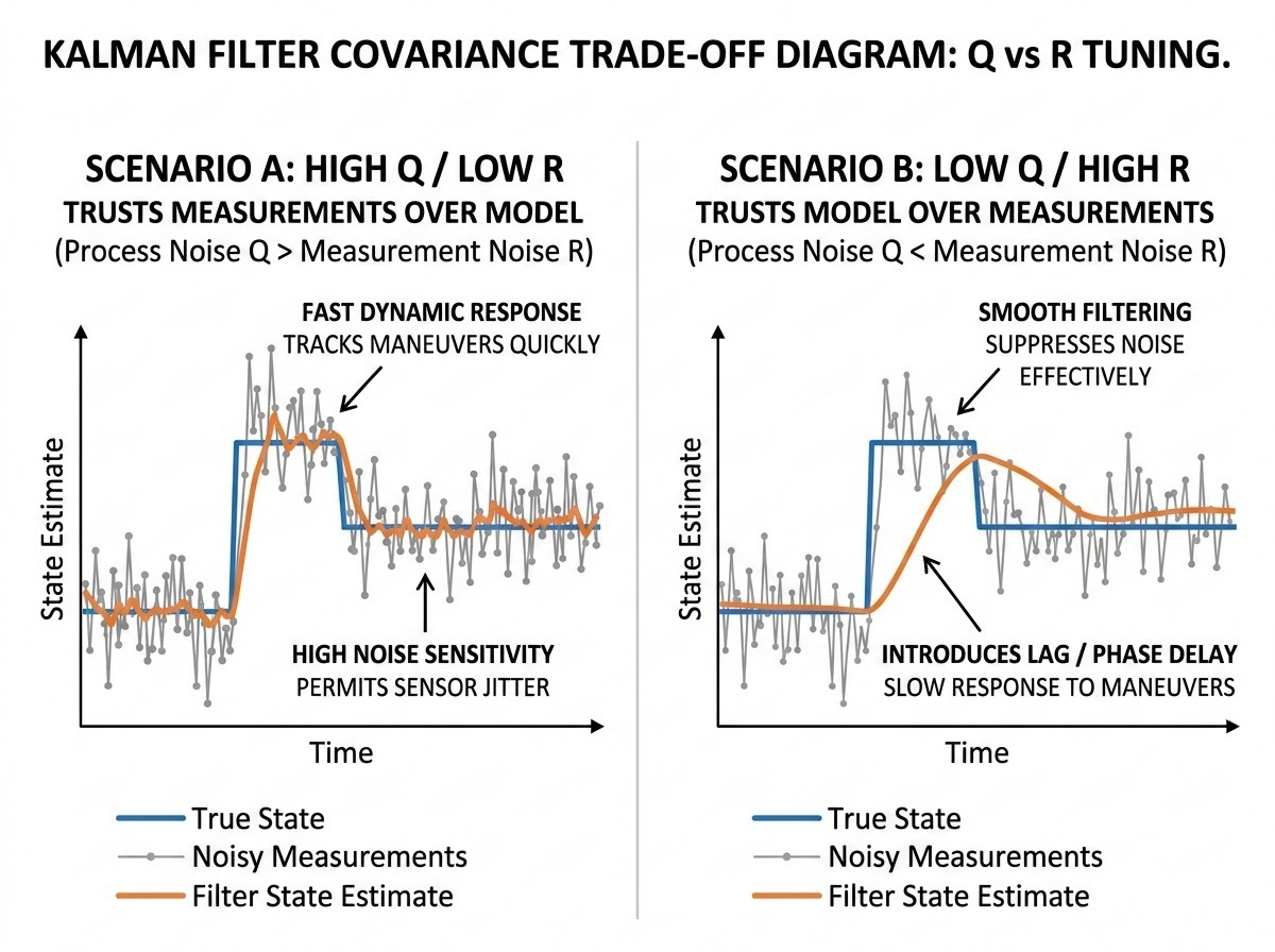
Diagram illustrating the trade-off between process noise covariance (Q) and measurement noise covariance (R) in a Kalman Filter. High Q / Low R leads to fast dynamic response and high noise sensitivity, tracking dynamic changes quickly but permitting sensor jitter. Low Q / High R results in smooth filtering and lag, suppressing noise effectively but introducing phase delay and slow response to maneuvers. — *Trade-off between process noise covariance (Q) and measurement noise covariance (R) in Kalman filter tuning.*

‍

A time-varying covariance can improve the result. Vibration indicators can increase accelerometer variance near a resonant rotor-speed band, while a magnetometer innovation gate can reject heading updates when field magnitude leaves its calibrated range. These solutions should be implemented before adding AI.

The remaining residual may still be systematic. Suppose the pitch error depends on motor speed squared, yaw rate, and measured vibration amplitude. A covariance change alone does not express that relationship. It changes confidence; it does not learn the correction function.

‍

Symbolic AI for Residual Correction and Data-Driven Modeling

Symbolic AI frames sensor drift mitigation as an analytical model discovery problem. Unlike black-box deep learning models, symbolic regression identifies explicit, human-readable mathematical expressions that map operating conditions to sensor residuals. This transparency allows control engineers to inspect model structure, verify physical constraints, and analyze stability prior to deployment 3.

OpenMathAI provides a visual environment supporting symbolic regression, state-space representations, and physics-informed neural networks (PINNs). Discovered symbolic models can be exported directly as ANSI C, FMU, or ONNX binaries for real-time integration onto platforms like the 3-DoF Copter 4, ensuring execution with minimal computational overhead on embedded microcontrollers.

‍

Learning a Correction Directly from Flight Data

The most defensible training target is not the absolute angle alone. It is the residual between an independent reference and the BNO055 output. On the 3-DoF Copter, encoder-derived pitch and yaw provide a practical reference for the corresponding mechanical angles, while the IMU supplies a separate sensor path. The reference is not perfect, so the experiment should document encoder resolution, synchronization, latency, and any geometric conversion used.

‍

‍

*OpenMathAI comes with pre-recorded sensor data, with various test conditions*

‍

*Recorded data shows both offset and drift between the ground truth (blue) and the IMU sensor data (orange)*

‍

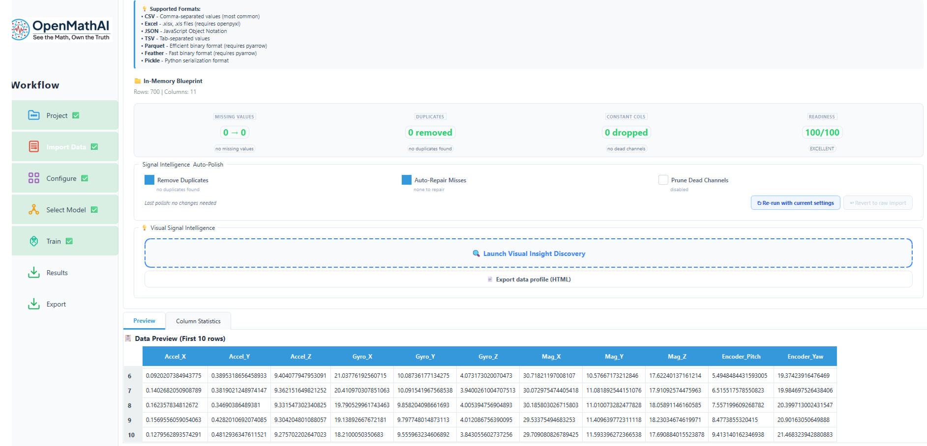
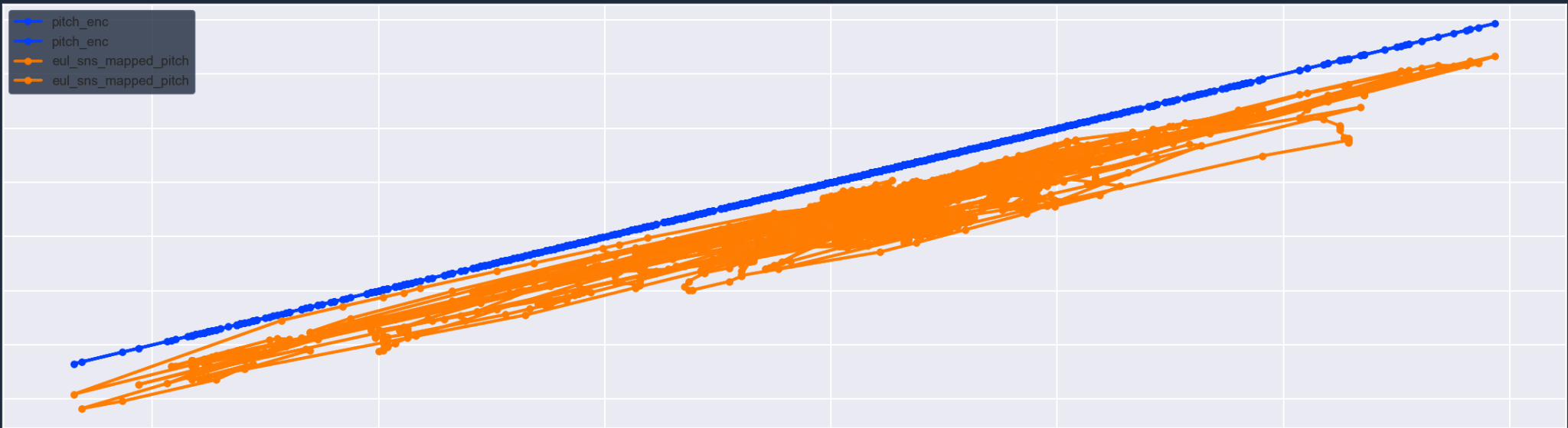
The target can be defined as:

e_pitch,k = θ_encoder,k - θ_IMU,k

and similarly for yaw. A symbolic model then estimates:

e_k = f(y_IMU,k, a_k, m_k, u_k, T_k, e_k-1)

The corrected estimate is:

θ_corr,k = θ_IMU,k + e_k

‍

The feature set should be constrained by causality. If the model is intended for real-time use, it must not use future samples. Lagged features, motor commands, and short-window vibration statistics are acceptable; a centered smoothing window is not.

Split by complete experiment runs rather than shuffled adjacent samples, and reserve unseen speeds and motion amplitudes for testing.

‍

Model Discovery and Interpretability

As shown below, OpenMathAI extracts explicit mathematical coefficients using dynamic lagged features (NARX structure) derived from logged time-series telemetries:

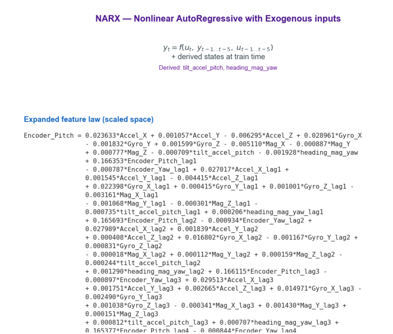
*OpenMathAI calculates the human-readable model coefficients and provides exports for different hardware output options*

‍

The core advantage of symbolic regression is structural interpretability: each term in the generated equation corresponds directly to physical phenomena, such as motor operating regimes, vibration amplitudes, or angular velocity dependencies. To prevent overfitting, parsimony penalties should be applied to constrain equation complexity. Simpler, dimensionally consistent equations yield higher robustness and safer bounded performance during closed-loop execution 3.

‍

Experimental Results and Comparative Analysis

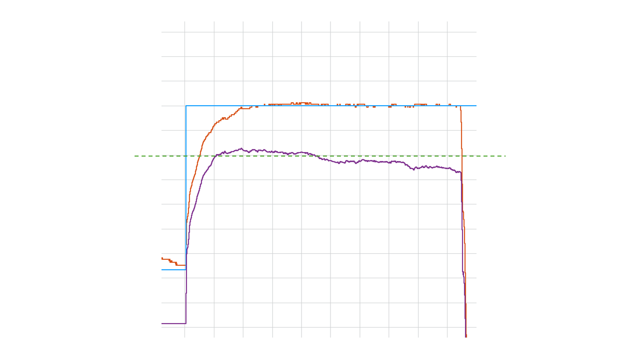
The following figures present an empirical comparison between a conventional Extended Kalman Filter (EKF) and the OpenMathAI-trained NARX (Nonlinear AutoRegressive with Exogenous inputs) symbolic model, evaluated against optical encoder ground-truth telemetry:

*Pitch and yaw estimation performance of a conventional EKF using 9-DoF IMU data versus encoder ground truth.*

‍

*Parity plots demonstrating high prediction accuracy and alignment with ground truth for the trained NARX Symbolic Model (R² = 0.9996).*

‍

*OpenMathAI residual distribution analysis confirming tight error bounds centered around zero.*

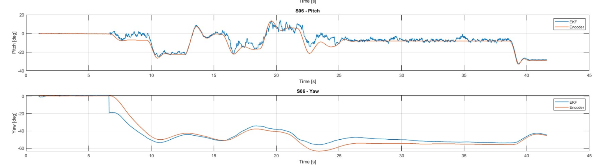
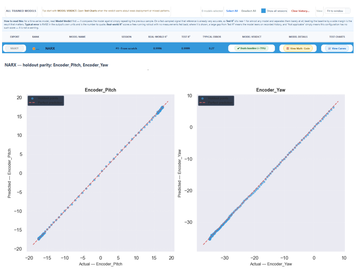
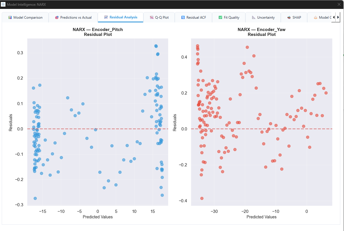
The table below summarizes the technical characteristics, operational requirements, and trade-offs between classical filtering and symbolic AI residual correction:

Kalman Filtering vs Symbolic AI Correction: A Comparison

‍

Method	Requires Known Noise Model	Explainability	Handles Nonlinear Vibration Coupling	Tuning Effort	Best For
Kalman Filter (EKF/UKF)	Yes, requires explicit process (Q) and measurement (R) noise models	High (explicit state-space formulation)	Limited, unless states and covariances are dynamically augmented	Manual covariance matrices, process models, and observability tuning	Real-time state estimation with known, Gaussian stochastic dynamics
Symbolic AI Correction	No, depends on representative telemetry data rather than noise priors	High when discovered analytical equations remain compact	High, maps errors to motor speed, vibration, and magnetic features	Dataset curation, feature selection, and parsimony constraints	Systematic, repeatable residuals tied to operational states
Hybrid Filter + Symbolic Residual	Combines physical baseline model with data-driven residual correction	High, provided each layer is documented and bounded independently	Optimal, combines stochastic state bounds with residual compensation	Highest, requires validating both filtering and learned residual layers	High-reliability control architectures and research applications

‍

In summary, while Kalman filtering provides a solid foundation for stochastic state estimation, Symbolic AI effectively captures complex, nonlinear residual errors driven by motor vibration and electromagnetic noise. Implementing a hybrid architecture leverages the advantages of both approaches, delivering superior estimation accuracy and robustness for real-time control applications.

‍

Running the Correction on the Acrome 3-DoF Copter

The Acrome platform is designed for real-time control education and research. Its published specifications include encoder and IMU feedback, a modular I/O architecture, MATLAB/Simulink compatibility, and courseware covering filtering, Kalman estimation, system modeling, and control design. That combination makes it suitable for a repeatable sensor drift correction experiment rather than a one-off benchtop demonstration.

A disciplined workflow has six stages. First, verify mechanical mounting, sensor axes, encoder sign conventions, timestamps, and calibration status. Second, collect stationary data with motors off and on. Third, collect controlled sweeps across motor commands and angular motion. Fourth, establish a conventional baseline using bandwidth selection, outlier rejection, and a Kalman filter. Fifth, train and validate the symbolic residual model using run-level splits. Sixth, deploy only a bounded and monitored version of the correction.

Also record peak error, phase lag, CPU time, memory use, saturation behavior, and closed-loop settling performance. Compare the original and corrected estimators side by side before increasing controller gains.

Disable the correction when calibration is invalid, the magnetic field leaves the training range, vibration exceeds the validated envelope, or the model produces an out-of-range value. These guards make the learned equation a bounded component rather than an unmonitored replacement for the sensor stack.

‍

Run this experiment on real hardware with the Acrome 3-DoF Copter, and correct its sensor drift with Vista1 Labs’ OpenMathAI, now available as a software option on the platform.

‍

For the coupled pitch and yaw dynamics behind this platform, see our MIMO Control System guide.

‍

Frequently Asked Questions

Why does the BNO055 IMU drift on the 3-DoF Copter?

The apparent drift can combine gyroscope bias, vibration-induced accelerometer error, magnetometer distortion from motor currents, temperature changes, and fusion-mode behavior. A calibration status of 3 does not prove that the output is unaffected by dynamic motor disturbances.

Is symbolic AI correction more accurate than a Kalman filter?

Not automatically. Symbolic correction can reduce a repeatable residual that the baseline filter does not model, especially when the error depends on motor operating point. A Kalman filter can remain superior when the plant and noise model are credible or when the data does not cover the operating envelope.

Do I need labeled ground truth data to train an OpenMathAI correction model?

You need a target that is more trustworthy than the signal being corrected. On a laboratory platform, synchronized encoder measurements can provide a practical reference for pitch and yaw. The reference’s resolution, latency, and mechanical alignment must be documented before training.

Can the corrected model run on the 3-DoF Copter’s own controller, or only offline?

That depends on the discovered model, controller interface, sample time, and deployment target. OpenMathAI describes code and model export options, but the resulting correction must be compiled, timed, range-checked, and validated on the actual real-time system before use in closed-loop control.

Does this replace Kalman filtering entirely, or work alongside it?

The safer default is to use it alongside a classical estimator. The Kalman filter can provide the state estimate and uncertainty handling, while the symbolic model supplies a bounded correction for a measured, repeatable residual. Removing the estimator requires a separate observability and stability analysis.

‍

Conclusion

Sensor drift correction is most valuable when the error is structured. If the BNO055 output changes with motor speed, vibration amplitude, magnetic field, or temperature, more aggressive low-pass filtering may reduce symptoms without explaining the cause. A conventional Kalman filter remains an essential baseline, but its covariance assumptions do not automatically capture every nonlinear hardware interaction.

A symbolic workflow adds a different capability. It can discover a compact residual equation from synchronized IMU, encoder, motor, and context data. The result can remain interpretable, constrained, and testable. It should not be trusted simply because its training error is low. Independent runs, physical plausibility checks, validity gates, and closed-loop tests are mandatory.

For researchers and lab teams who want to study this problem on repeatable hardware, the Acrome 3-DoF Copter provides the plant, feedback paths, real-time interfaces, and control-system context. OpenMathAI can then be evaluated as the data-driven layer in a broader sensor fusion experiment. The strongest result is not “AI replaces filtering.” It is a measured hybrid architecture in which each model has a clear job and a verifiable limit.

‍